Customizing Civil 3D Reports (XSL Report Customizing)

Have you ever wanted to customize a Civil 3D Report? Perhaps you like how a report looks but need to add some additional content. This post will get into the extended functionality that allows you to customize your Civil 3D Reports. To warn you ahead of time, customizing the reports does require some programming knowledge, however, the level of programming knowledge required depends on the report.

To begin, let's first take a look at the Toolspace Toolbox where the Reports can be found

Toolspace Toolbox
When you look at the Toolspace Toolbox you will find multiple locations of reports. The first set of reports under Reports Manager is the section that I'm focusing on in this blog post, but let's briefly discuss the others as well.

Reports under Report Manager
These reports have been shipping with Civil 3D since it's debut, at least as far back as I can remember first using Civil 3D in 2007/2008.

Miscellaneous Utilities - Reports
These reports have been added over the years as Civil 3D has been improving. From my understanding, these reports have limited to no customization available. However, there are some really great and useful reports in here that you may find beneficial, so have a look when you have some time.

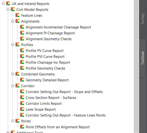
Country Kits Reports
If you have any Country Kits installed, you may or may not find additional reports here. In my case, I have the UKIE Country Kit installed and there are a good number of additional reports provided here - some are very useful reports!

Customizing the Reports Manager Reports

Before we get into the deep end of customizing the reports, it's important to cover the basic settings of how the reports work.

Above Reports Manager, there are two buttons.

The left button launches a dialog that allows you to edit Company, Client, Project information about the report you will be generating. ImaginIt has a good blog post on how this work here. However, what's not stated is if you want to push this out to all of your users with standard information, you need to know where the data is saved. You can find it at this path:

C:\Users\$username%\AppData\Local\Autodesk\LandXML Reporting\RepGenConfig.xml

The right button launches the Toolbox editor that allows you to add your own custom directories for your personalized/company standard reports. These can be manually added for ease of finding in the future. However, again, how do you push this out to users? Christopher Fugitt with Civil 3D Reminders has a great post on how to do that here.

Determining How the Report was Created

Now that we have the basics covered let's start with how one can customize the reports.

First you'll need to determine how the report was written so that you can find the code project. The reports written and executing from the Reports Manager have two formats DLL and XSL, though I don't believe you are limited to just these two if you have a working report say written in VBA. It is important to understand what these two file formats provided are and how they are created before we proceed further, therefore:

What is a DLL file? from support.microsoft.com

"A DLL is a library that contains code and data that can be used by more than one program at the same time."

These files are the compiled code output from an Integrated Development Environment (IDE) such as Visual Studio. The DLL file cannot be directly opened and viewed, but requires the actual code project where one can edit the code and recompile the DLL file for use. The DLL could be compiled from a number of different language types, but for AutoCAD Civil3D, you're more likely to find C#.NET or vb.NET languages.

What is an XSL file? from w3.org

"XSL is a language for expressing style sheets. An XSL style sheet is, like with CSS, a file that describes how to display an XML document of a given type."

XSL files can be opened, viewed and edited much easier than a DLL can. For those that are familiar HTML and CSS, you'll find similar formatting within the XSL file. This file could be opened and edited with a number of different programs, but the two I would recommend are Notepad++ or VisualStudio Code.

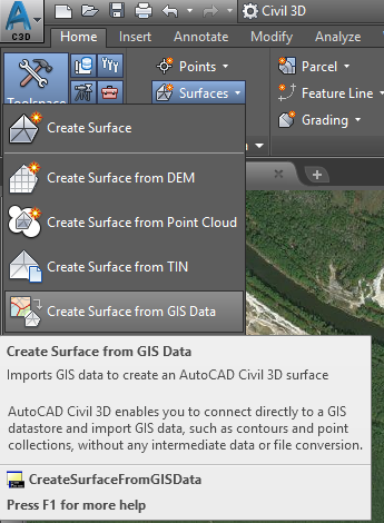
Inspect the Incremental Station Elevation Difference Report

If we browse into Reports Manager / Profile / Incremental Station Elevation Difference Report and located the Macro / Executing File, you'll see that it ends with C3D Report.dll.

 

This means this report is written in a format that will be more advanced level of programming to try and edit it. While I won't be getting into how to edit this report, I can tell you it is written in .NET and the code project can be found at the path below for a seasoned developer to get in, make some changes and recompile the DLL for use of Civil 3D users.

C:\ProgramData\Autodesk\C3D YEAR\enu\Data\Reports\Net\Source

Inspect the Profiles_in_CSV Report
If we browse into Reports Manager / Profile / Profiles_in_CSV Report and located the Macro / Executing File, you'll see that it ends with profileCSV.xsl.

You can find the file for this report in the following path and use Notepad++ or VisualStudio Code to make your edits. Let's get in and break down what happens with an XSL report file.

C:\ProgramData\Autodesk\C3D YEAR\enu\Data\Reports\xsl

Breaking Down XSL Reports
Recall that XSL is a style sheet applied to an XML file. When you execute any of the XSL reports the first thing that happens is the LANDXMLOUT command is executed and the LandXML file is read into memory. The XSL report then takes over and reads through the LandXML output to extract data from the LandXML and format it into a easily readable report.

If you open up the Profiles_in_CSV.xsl file, we can break down what the code is doing. It's important to recognize that the XSL file is reading from a number of other XSL files. This is because the file is calling functions that are stored in other files. The functions (written in JSON) either set or get data. We'll take a look at that a bit later, but for now, just note that there are other XSL files involved here.

Next, there are 3 main sections of the code - I'll call them: Match "/", Match "lxAlign", and Match "lxProfAlign"

Match "/"
In this section, it is looking through the entire XML file for "PVI", "grade out (%)", and lastly . The first two are gathering those string sections to make a choice on units and formatting of units. The last section is using the string " " to select each alignment, this passes the alignment to the next section.

 

Match "lxAlign"

This section loops through the alignment and gets the lx:ProfAlign to pass to the next section. It also performs some station equations - I believe to ensure there are no differences in stationing between the profile and the alignment, perhaps due to how LandXML outputs the data from Civil 3D.

 

Match "lxProfAlign"
This section is what actually populates the report. Notice that this section loops through all the PVIs in the profile. There are three parts to this section - the first is getting the node number, second is storing data into variables that reference the node number, and the last is passing the variables to a number format function.

Node Number
The node number is each PVI in the profile. The number is stored in a variable like this

xsl:variable name="number" select="position()"

where "number" is the variable name and it's returning it's position

Variables
The variables are defined and the functions are called with the node number like this

xsl:variable name="elev" select="landUtils:GetVElevation($number)"

where "elev" is the variable name and it's the number variable with $number into a function called GetVElevation. If we locate this function, we will see that it is returning the elevation of the PVI based on it's number within the profile.

Formatting

Lastly the variables are passed to the number formatting function which formats the number to a specific format for output on the report. It's passing each like this:

FormatNumber(string($elev), string($SourceLinearUnit), string($Profile.Elevation.unit), string($Profile.Elevation.precision), string($Profile.Elevation.rounding))"

In the above case it's passing the variable "elev" as $elev and also passing some stored settings from the Match "/" section discussed above to tell the function how to format the value.

For further breakdown, we need to open up the referenced XSL files first mentioned when opening the report XLS file.

XSL References
Recall the references used by Profiles_in_CSV.xsl. Let's take a look at each of these.

Open Header.xsl
When we open up Header.xsl, note that it is also refencing Text_Formatting.xsl, but overall this document simply sets up a standard header that is used in all of the reports. The information here is pulling from the ..\LandXML Reporting\RepGenConfig.xml mentioned in the beginning of this blog post. Some formatting settings are being passed into the Number_Formatting.xsl document so that when it's functions are called they output the report the way you'd like it too look.

Open V_Alignment_Layout_b.xsl
This document contains the functions that are returning the alignment and profile data. The functions are written in JSON and there are quite a few in here that may or may not be used by the example report discussed in this post. You can find the functions by looking for function, as shown below. Then you can see the function name, in this case "GetVEndStation". For some functions, they require something to be passed into them and this is defined within the parenthesis.

function GetVEndStation()

Breakdown a Function
Let's look at a function. Below you can see the function "GetVElevation". Within the parenthesis it's asking for an index number. In this situation, this is asking for a PVI number, if you recall from earlier in the post.

Next, in JSON the variable is defined as "var" and they give the name of "ndx". From here it passes the index value into a JSON number function that simply converts a string to a number. This is then passed into the "VElementArray", which is the entire profile stored in memory from the LandXML and obtains the PVI by it's number - which is stored as a variable called "ele". Finally it returns the Elevation of the PVI.

function GetVElevation(index)
{
    var ndx = Number(index);
    var ele = VElementArray[ndx];
   
    return ele.Elevation;
}

Open Number_Formatting.xsl

This document contains a lot of JSON functions that convert values to different formatting, include numeric values into stationing formats. The start of the file has a number of defined parameters that are established at runtime of the report from the Header file as it's passing in the stored settings of the Report Manager.

Example

Let's add a variable and add it to the Profiles_in_CSV.xsl report. Here I've added two variables for "crvStrt" and "crvEnd" that call functions for GetPVCStation and GetPVTStation, then this data will be output to the report through the number formatting functions.

When you execute the report - the Event Viewer will tell you if the report did not run and why. You do need to be careful with your code to make sure there are not any typos as there's no notifications on this from Notepad++ or VisualStudio Code.

What Does All This Mean?

That was a lot of information that we just covered, so what does it all mean? For XSL reports, it means there's already a numerous written functions in JSON that can be referenced in your reports. It also means for a seasoned JSON developer, additional functions could be written. You can copy functions and perform mathematics on them if you'd like as well to output specialized data in your reports as needed. It's all coming from the export LandXML files directly from your Civil 3D files and is a great way to parse out the data into a presentable report.

In this blog post I've only shown you a small portion of what functions are in the XSL files. You'll have to do some searching to determine what's all there to suit your needs, but I hope you now have a better understanding of these reports and how they can be customized.

Zoom to Extents of All Objects On a Layer

I recently had someone ask me if there was a way to quickly zoom to all objects on a specific layer. I couldn't find any written LISP code as a whole, but found some small pieces here and here that I was able to utilize and make a command to do this.

Load up this lisp, and then run ZOLAYER to pick an object and zoom to the extents of all objects on that layer. Enjoy!

LISP CODE
====================================================================
(defun SALL ()
(setq TargEnt (car (entsel "\nSelect object on layer to select: ")))
(setq TargLayer (assoc 8 (entget TargEnt)))
(sssetfirst nil (ssget "_X" (list TargLayer)))
(princ)
);defun

(defun ZOE ()
(if (setq ss1 (ssget "_I"))
(command "ZOOM" "OBject" ss1 "")
(command "ZOOM" "Extents")
);if
);defun

(defun c:ZOlayer ()
(SALL)
(command)
(command)
(ZOE)
);defun
=======================================================================

Leveraging GIS Data in Civil 3D: Querying Data Between Files

Following up on last week's post on Leveraging GIS Data in Civil 3D, this week I'm covering how to query data between drawing files using Civil 3D's built in Map functionality. As I mentioned in the previous post, this blog post also applies to Map 3D software as a stand alone and to the new 2019 AutoCAD Only One with the Map extension added in.

To begin, I already have a drawing file setup with GIS data from a county source. This file can be in whatever coordinate system deemed necessary to match the data and I had used the MAPIMPORT command explained in the previous blog post.

 

However, when clicking on contours, you can see that the AutoCAD property of the contours do not read the proper information from the Object Data table, thus in this post I'll demonstrate how to query the data over to a new drawing file on the same or a different coordinate system, apply a spatial filter, and alter the AutoCAD properties of the objects to inherit the Object Data information.

For this example, I am using the Elevation property, but this can be done for almost any of the AutoCAD properties about the objects.

 

In a new drawing, I've setup my project coordinate system and brought in the Bing imagery for my site and located where I wanted contour data. At the bottom of my screen you can see the coordinate system. By the way, by default this coordinate system in the status bar is turned off by default. To turn this on, you can use the command MAPSTATUSBAR.

 

 Next, to use the Map querying functionality, we need to turn on the Map Task Pane. Use the command MAPWSPACE to turn this on. You should see something like below.

 

Using the MapExplorer tab of the Map Task Pane, right click on drawing and select Attach...

 

 On the select drawing to attach dialog, you'll find that this is not as simple to use as other dialogs. Essentially you have to setup a drive alias to your file(s) location and then tell this dialog to look at that drive alias. To do this, select the button circled in red below.

 Here you'll need to setup the drive alias and browse to your actual path. Then select Add to add the alias to the drive list. Select close when done.

 

 Now on the Select drawings to attach dialog, you should be able to select your drive alias and it will take you to your file(s) location.

Find the drawing(s) you would like to reference, and select Add. The drawing(s) will be added to a list. Select Ok when done.

 

In the Map Task Pane, you should now see your drawing attached. It's important to note that when doing this, the file is opened and a file lock is placed on the file. Once completed, you will need to make sure the file(s) are detached to release the locks.

 

 

Next, we are ready to define our query of data, thus on the Map Task Pane, on Map Explorer tab, locate Query Library and right click, select Define.

 

The dialog below will appear to allow you to build your query. The top white box is your current query information. The bottom left Query type allows you to query a location of the drawing(s), specific object property information, Data, and SQL calls on the tables. Query Mode allows you to Preview, Draw, or Report on the query. Options allows you to do some additional items like altering properties.

For this example, let's start by selecting the Location... button.

 

Here you'll be prompted to select your Location Condition. For Boundary type I'll use Boundary, with a selection type of Inside. This should bring in the data inside a selected Polyline. If you want all the data, just choose All. For some of the boundary options like Polyline and Window, you'll need to select the Define button at the bottom and the define the area or object. Select ok when done.

 

Next, you'll be back on the Define query dialog. Choose Properties. Here we'll tell it to only look at objects on a specific layer. We can choose layer, then Values, and select our layer. Choose Ok.

 

Back on the Define query dialog, we now want to specify what properties we would like to alter. Select the Alter Properties button. Here you can alter many properties at once. The white box at the top of the dialog shows your Current Property Alterations. Below that you have options of what you would like to alter (FYI, you can even alter Text to display specific object data property information!).

For this example, we'll choose Elevation, and then choose the Expression button. The expression dialog will appear and we'll need to select the corresponding Object Data Table and property we want to pass over. In this case it's the Walton_Contours, ContourElev property. Select Ok on the Expression dialog.

 

You should now see your expression like shown below. Click Add to add this to your current property alterations.

 

The property alterations dialog will now show the information like below. Either add more properties to alter, or choose Ok when done.

 

Back on the Define Query dialog, we should see something like below. Be sure to set the Query mode to Draw, and make sure the Checkbox in Options next to the Alter Properties is checked. This controls whether the Alter Properties runs or not. Choose Execute Query when done.

 

The contour data should now come over and when selecting a contour you can see the Object Data table information has been applied to the AutoCAD elevation property... for every contour in your query! Again, this can be done for many objects and properties all at once and could be very helpful to translate your GIS data appropriately.

 

Lastly, as I mentioned earlier, be sure to detach your file from the Map Task Pane to ensure it is unlocked for others to use.

It's important to note that this is just an example of one type of data. The options here are nearly endless with the what data you are using and what can be queried and fully brought into functional AutoCAD objects from GIS data referencing the GIS Object Data tables. It's also important to note that I am not aware of any ways to apply GIS Object Data to Civil 3D objects - the Alter Properties only works with the AutoCAD Properties available and does not allow for extended Civil 3D information - nor does it allow for access to Property Sets which I believe could be beneficial for Civil 3D 2017 and greater which provides access and labeling of Property Sets.

Leveraging GIS Data in Civil 3D

When utilizing GIS data on a Civil 3D project, one should first ask themselves some questions regarding the data in order to handle processing the data in the most efficient manor. I like visuals for systems thus I've created this flowchart using Autodesk's Praxis Workflow Editor here.

Ultimately in this post, I will explain the four primary method's for importing GIS data in Civil 3D.

1. Static Connection using MAPIMPORT
2. Dynamic Connection using FDO
3. Create Surface from GIS Data
4. Import GIS Data (Pipe Networks)

First, I think it's helpful to note that GIS data processing commands are distributed with Civil 3D but are not actually a part of Civil 3D - they belong to another piece of Autodesk software called AutoCAD Map 3D. This is helpful to know when you are searching for help documentation on commands and to understand that much of what I'll be posting below applies to AutoCAD Map 3D users as well. And for those moving to 2019 products, we have the exciting news of Only One. AutoCAD. in which we can now get specific toolsets added to AutoCAD to help workflows; AutoCAD Map 3D Toolset being one of those.

1) Static Connection MAPIMPORT Command

The MAPIMPORT command is used for bringing in data in static form into your drawing and can be accessed by typing the command syntax MAPIMPORT. The result is importing as AutoCAD objects as well which usually provides the best results in formatting the data with the normal AutoCAD controls for displaying on drawings.

Upon running the command, you are first prompted for the file. The MAPIMPORT command has many different file types it supports, but for this example we have a simple SHP file and thus will choose ESRI Shapefile (*.SHP).

The next dialog will show your current drawings' assigned coordinate system (highlighted in red) - if you forgot to assign one, you can do so by clicking the globe button without exiting the command. The spatial filter area allows you to clip the data to a specific area, should your drawing be setup already in a way that you can correct select the spatial location. Each file selected will appear in the Import Properties section of the dialog where you can assign the layer of the object and verify the coordinate system of the file (highlighted in blue). Note that if the drawing and the file have differing coordinate systems, the software will translate the file data to the current drawing's coordinate system.

Next is the data attached to the file. If you want to be able to view the extended object data, it's important to click into the data column for each file and select the '...' button to choose the option to Create Object Data. You can then also specify which fields are brought over.

Lastly, when using this option, I prefer to Import Polygons as closed Polylines.

Here is the result of this shape file that contained data for the countries of Africa and how the data came in. Note that upon selecting any objects and viewing the AutoCAD properties, there is a section for Object Data in which you'll be able to view the extended info about that object.

2) Dynamic Connection Using FDO

The FDO  option provides a dynamic link to the data which is important if the data will be updating regularly throughout your project. To access this option, you must first access the Map3D portion of Civil 3D using the Map Task Pane. To do this from the Civil 3D workspace, type in the command syntax MAPWSPACE and choose to turn the Task Pane On. The palette below will appear.

Click on Data (highlighted in red) and choose Connect to Data...

 The Data Connect Palette will appear showing all the different methods of connecting to data. For this SHP file, we'll use the Add SHP Connection, then choose either the SHP file button or the folder button.

 Once choose, select the Connect button.

 The SHP file(s) will be added as connections and show up in the sources. To add them to your current drawing, select them and choose Add to Map.

Below you can see the same SHP file brought in, though the default appearance looks drastically different. Note when choose the objects and viewing in properties, they show as Map Features. These cannot be formatted using the native AutoCAD methods.

 To format the appearance, note that you can see these in your Map Task Pane. Right click on the item and choose edit style. From here you can use the Map method of formatting how the objects appear.

 

Any changes to the data on the GIS side will then be reflected into your drawing automatically.

3) Static Connection: Create Surface From GIS Data Command

To streamline the process of importing surface data and generate a Civil 3D surface, we can use the Create Surface from GIS Data command found on the Home Tab, Surfaces drop down or use the command syntax CreateSurfaceFromGISData.

 The object options tab will provide you the ability to name the surface and set it's style.

Next you'll connect to the data type file or folder, and select Login button.

 Next you'll see the schema available in the selected file along with the coordinate system assigned to the file and the coordinate system of your drawing. This command will translate the data as necessary.

 On the Geospatial Query tab we can filter the data to a selected are on the drawing if you already know where your site lies.

 Lastly, on the Data Mapping tab, you need to specify what data in the file is the relevant Civil 3D Elevation property - in this case the elevation data is stored as ContourEle within the SHP file.

 Selecting finish will then generate a surface from the selected file in which we can then use as our normal Civil 3D surfaces. More information on this command can be found at this AKN.

4) Static Connection: Import GIS Data Command

Autodesk should really be relocated under the Home tab Create Pipe Networks and should be called Create Pipe Network From GIS data as that's ultimately what it is meant to do. But for now, to access this command, go to the Insert tab, Import panel, and select the drop down. Choose Import GIS Data or use the command syntax _AeccImportGISData

You'll be prompted to select the SHP file or path to SHP files, then follow the steps through wizard to map the data to the corresponding properties.

 On the Object Options tab you'll name the Civil 3D Pipe Network, select a Parts List and labels.

 On the Schema and Coordinates tab, you'll see your SHP files and if it's able to show the coordinate system of the data it would populate correctly - for this example, these files will need some additional work to assign the coordinate system with ArcGIS. At the bottom of this tab page you can also set your drawing's coordinate system.

For Data Mapping: Pipes, you'll need to look at the available feature classes in the SHP file and select what cross sectional shape to apply to the pipes. Click add to apply that shape to the feature class.

 Once added, then you'll need to assign attributes from the SHP file to the Civil 3D properties. This is where you'll need to fully understand the Schema used in the object data for the SHP file to know what to choose for the various components of the Civil 3D pipes. Critical items will be material, diameter, start location, end location, and elevations, but you may have other data helpful for mapping.

The same process will be applied for structures on the Data Mapping: Structures tab.

 With the Query Options tab, you'll be able to limit how much of the SHP file is brought into Civil 3D. This can significantly speed up the process of bringing in the data depending on how many pipes and structures are in the SHP files.

 Lastly is the Cleanup tab in which you can force snap tolerances for pipes and structures and also discard any data that is unlinked to pipes/structures.

Ultimately, bringing the data in you'll have a Civil 3D Pipe Network with the proper locations, elevations, materials, and other data assigned from the SHP file. For more information, see this AKN.





In my next post, I plan to follow with utilizing the AutoCAD Map 3D's ability to query data between drawings on different coordinate system and how we can leverage that to easily exchange data between files.